Machine learning models have become an integral component of decision-making across multiple industries, yet they often encounter difficulty when dealing with noisy or diverse data sets. That is where Ensemble Learning comes into play.
This article will demystify ensemble learning and introduce you to its powerful random forest algorithm. No matter if you are a data scientist looking to hone your toolkit or a developer looking for practical insights into building robust machine learning models, this piece is meant for everyone!
By the end of this article, you will gain a thorough knowledge of Ensemble Learning and how Random Forests in Python work. So whether you are an experienced data scientist or simply curious to expand your machine-learning abilities, join us on this adventure and advance your machine-learning expertise!
Ensemble learning is a machine learning approach in which predictions from multiple weak models are combined with each other to get stronger predictions. The concept behind ensemble learning is decreasing the bias and errors from single models by leveraging the predictive power of each model.
To have a better example let’s take a life example imagine that you have seen an animal and you do not know what species this animal belongs to. So instead of asking one expert, you ask ten experts and you will take the vote of the majority of them. This is known as hard voting.
Hard voting is when we take into account the class predictions for each classifier and then classify an input based on the maximum votes to a particular class. On the other hand, soft voting is when we take into account the probability predictions for each class by each classifier and then classify an input to the class with maximum probability based on the average probability (averaged over the classifier’s probabilities) for that class.
Ensemble learning is always used to improve the model performance which includes improving the classification accuracy and decreasing the mean absolute error for regression models. In addition to this ensemble learners always yield a more stable model. Ensemble learners work at their best when the models are not correlated then every model can learn something unique and work on improving the overall performance.
Although ensemble learning can be applied in many ways, however when it comes to applying it to practice there are three strategies that have gained a lot of popularity due to their easy implementation and usage. These three strategies are:
- Bagging: Bagging which is short for bootstrap aggregation is an ensemble learning strategy in which the models are trained using random samples of the data set.
- Stacking: Stacking which is short for stacked generalization is an ensemble learning strategy in which we train a model to combine multiple models trained on our data.
- Boosting: Boosting is an ensemble learning technique that focuses on selecting the misclassified data to train the models on.
Let’s dive deeper into each of these strategies and see how we can use Python to train these models on our dataset.
Bagging takes random samples of data, and uses learning algorithms and the mean to find bagging probabilities; also known as bootstrap aggregating; it aggregates results from multiple models to get one broad outcome.
This approach involves:
- Splitting the original dataset into multiple subsets with replacement.
- Develop base models for each of these subsets.
- Running all models concurrently before running all predictions through to obtain final predictions.
Scikit-learn provides us with the ability to implement both a BaggingClassifier and BaggingRegressor. A BaggingMetaEstimator identifies random subsets of an original dataset to fit each base model, then aggregates individual base model predictions?—?either through voting or averaging?—?into a final prediction by aggregating individual base model predictions into an aggregate prediction using voting or averaging. This method reduces variance by randomizing their construction process.
Let’s take an example in which we use the bagging estimator using scikit learn:
from sklearn.ensemble import BaggingClassifier
from sklearn.tree import DecisionTreeClassifier
bagging = BaggingClassifier(base_estimator=DecisionTreeClassifier(),n_estimators=10, max_samples=0.5, max_features=0.5)
The bagging classifier takes into consideration several parameters:
- base_estimator: The base model used in the bagging approach. Here we use the decision tree classifier.
- n_estimators: The number of estimators we will use in the bagging approach.
- max_samples: The number of samples that will be drawn from the training set for each base estimator.
- max_features: The number of features that will be used to train each base estimator.
Now we will fit this classifier on the training set and score it.
bagging.fit(X_train, y_train)
bagging.score(X_test,y_test)
We can do the same for regression tasks, the difference will be that we will be using regression estimators instead.
from sklearn.ensemble import BaggingRegressor
bagging = BaggingRegressor(DecisionTreeRegressor())
bagging.fit(X_train, y_train)
model.score(X_test,y_test)
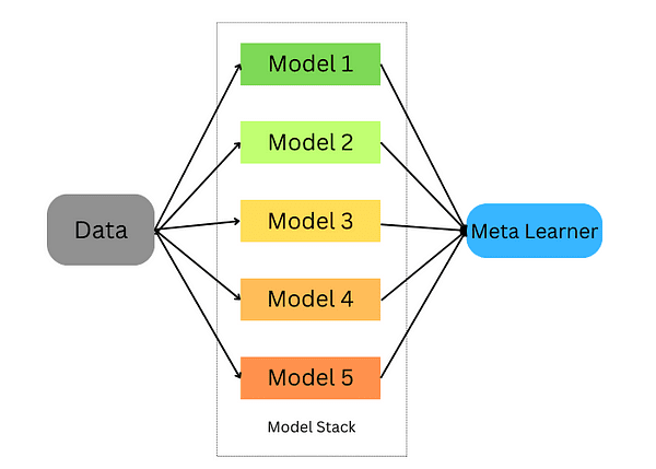
Stacking is a technique for combining multiple estimators in order to minimize their biases and produce accurate predictions. Predictions from each estimator are then combined and fed into an ultimate prediction meta-model trained through cross-validation; stacking can be applied to both classification and regression problems.

Stacking ensemble learning
Stacking occurs in the following steps:
- Split the data into a training and validation set
- Divide the training set into K folds
- Train a base model on k-1 folds and make predictions on the k-th fold
- Repeat until you have a prediction for each fold
- Fit the base model on the whole training set
- Use the model to make predictions on the test set
- Repeat steps 3–6 for other base models
- Use predictions from the test set as features of a new model (the meta model)
- Make final predictions on the test set using the meta-model
In this example below, we begin by creating two base classifiers (RandomForestClassifier and GradientBoostingClassifier) and one meta-classifier (LogisticRegression) and use K-fold cross-validation to use predictions from these classifiers on training data (iris dataset) for input features for our meta-classifier (LogisticRegression).
After using K-fold cross-validation to make predictions from the base classifiers on test data sets as input features for our meta-classifier, predictions on test sets using both sets together and evaluate their accuracy against their stacked ensemble counterparts.
# Load the dataset
data = load_iris()
X, y = data.data, data.target

# Split the data into training and testing sets
X_train, X_test, y_train, y_test = train_test_split(X, y, test_size=0.2, random_state=42)

# Define base classifiers
base_classifiers = [
   RandomForestClassifier(n_estimators=100, random_state=42),
   GradientBoostingClassifier(n_estimators=100, random_state=42)
]

# Define a meta-classifier
meta_classifier = LogisticRegression()

# Create an array to hold the predictions from base classifiers
base_classifier_predictions = np.zeros((len(X_train), len(base_classifiers)))

# Perform stacking using K-fold cross-validation
kf = KFold(n_splits=5, shuffle=True, random_state=42)
for train_index, val_index in kf.split(X_train):
   train_fold, val_fold = X_train[train_index], X_train[val_index]
   train_target, val_target = y_train[train_index], y_train[val_index]

   for i, clf in enumerate(base_classifiers):
       cloned_clf = clone(clf)
       cloned_clf.fit(train_fold, train_target)
       base_classifier_predictions[val_index, i] = cloned_clf.predict(val_fold)

# Train the meta-classifier on base classifier predictions
meta_classifier.fit(base_classifier_predictions, y_train)

# Make predictions using the stacked ensemble
stacked_predictions = np.zeros((len(X_test), len(base_classifiers)))
for i, clf in enumerate(base_classifiers):
   stacked_predictions[:, i] = clf.predict(X_test)

# Make final predictions using the meta-classifier
final_predictions = meta_classifier.predict(stacked_predictions)

# Evaluate the stacked ensemble's performance
accuracy = accuracy_score(y_test, final_predictions)
print(f"Stacked Ensemble Accuracy: {accuracy:.2f}")
Boosting is a machine learning ensemble technique that reduces bias and variance by turning weak learners into strong learners. These weak learners are applied sequentially to the dataset; firstly by creating an initial model and fitting it to the training set. Once errors from the first model have been identified, another model is designed to correct them.
There are popular algorithms and implementations for boosting ensemble learning techniques. Let’s explore the most famous ones.
6.1. AdaBoost
AdaBoost is an effective ensemble learning technique, that employs weak learners sequentially for training purposes. Each iteration prioritizes incorrect predictions while decreasing weight assigned to correctly predicted instances; this strategic emphasis on challenging observations compels AdaBoost to become increasingly accurate over time, with its ultimate prediction determined by aggregating majority votes or weighted sum of its weak learners.
AdaBoost is a versatile algorithm suitable for both regression and classification tasks, but here we focus on its application to classification problems using Scikit-learn. Let’s look at how we can use it for classification tasks in the example below:
from sklearn.ensemble import AdaBoostClassifier
model = AdaBoostClassifier(n_estimators=100)
model.fit(X_train, y_train)
model.score(X_test,y_test)
In this example, we used the AdaBoostClassifier from scikit learn and set the n_estimators to 100. The default learn is a decision tree and you can change it. In addition to this, the parameters of the decision tree can be tuned.
2. EXtreme Gradient Boosting (XGBoost)
eXtreme Gradient Boosting or is more popularly known as XGBoost, is one of the best implementations of boosting ensemble learners due to its parallel computations which makes it very optimized to run on a single computer. XGBoost is available to use through the xgboost package developed by the machine learning community.
import xgboost as xgb
params = {"objective":"binary:logistic",'colsample_bytree': 0.3,'learning_rate': 0.1,
               'max_depth': 5, 'alpha': 10}
model = xgb.XGBClassifier(**params)
model.fit(X_train, y_train)
model.fit(X_train, y_train)
model.score(X_test,y_test)
3. LightGBM
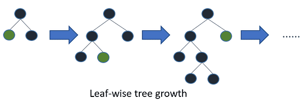
LightGBM is another gradient-boosting algorithm that is based on tree learning. However, it is unlike other tree-based algorithms in that it uses leaf-wise tree growth which makes it converge faster.

Leaf-wise tree growth / Image by LightGBM
In the example below we will apply LightGBM to a binary classification problem:
import lightgbm as lgb
lgb_train = lgb.Dataset(X_train, y_train)
lgb_eval = lgb.Dataset(X_test, y_test, reference=lgb_train)
params = {'boosting_type': 'gbdt',
             'objective': 'binary',
             'num_leaves': 40,
             'learning_rate': 0.1,
             'feature_fraction': 0.9
             }
gbm = lgb.train(params,
   lgb_train,
   num_boost_round=200,
   valid_sets=[lgb_train, lgb_eval],
   valid_names=['train','valid'],
  )
Ensemble learning and random forests are powerful machine learning models that are always used by machine learning practitioners and data scientists. In this article, we covered the basic intuition behind them, when to use them, and finally, we covered the most popular algorithms of them and how to use them in Python.
Youssef Rafaat is a computer vision researcher & data scientist. His research focuses on developing real-time computer vision algorithms for healthcare applications. He also worked as a data scientist for more than 3 years in the marketing, finance, and healthcare domain.

