Pooling layers are common in CNN architectures used in all state-of-the-art deep learning models. They are prevalent in Computer Vision tasks including Classification, Segmentation, Object Detection, Autoencoders and many more; simply used wherever we find Convolutional layers.
In this article, we’ll dig into the math that makes pooling layers work and learn when to use different types. We’ll also figure out what makes each type special and how they are different from one another.
Pooling layers provide various benefits making them a common choice for CNN architectures. They play a critical role in managing spatial dimensions and enable models to learn different features from the dataset.
Here are some benefits of using pooling layers in your models:
All pooling operations select a subsample of values from a complete convolutional output grid. This downsamples the outputs resulting in a decrease in parameters and computation for subsequent layers, which is a vital benefit of Convolutional architectures over fully connected models.
Pooling layers make machine learning models invariant to small changes in input such as rotations, translations or augmentations. This makes the model suitable for basic computer vision tasks allowing it to identify similar image patterns.
Now, let us look at various pooling methods commonly used in practice.
For ease of comparison let’s use a simple 2-dimensional matrix and apply different techniques with the same parameters.
Pooling layers inherit the same terminology as the Convolutional Layers, and the concept of Kernel Size, Stride and Padding is conserved.
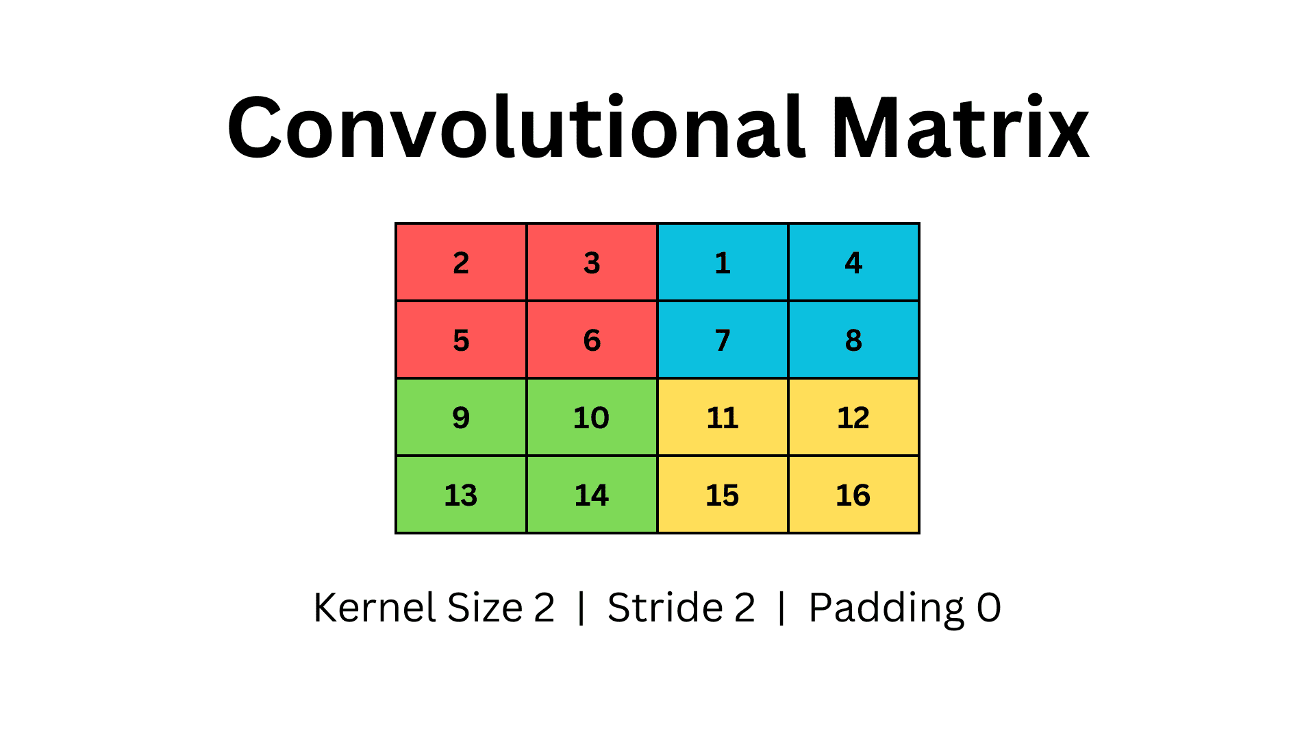
So, here we define a 2-D matrix with four rows and four columns. To use Pooling, we will use a Kernel size of two and stride two with no padding. Our matrix will look as follows.

Image by Author
It is important to note that pooling is applied on a per-channel basis. So the same pooling operations are repeated for each channel in a feature map. The number of channels remains invariant, even though the input feature map is downsampled.
We iterate the kernel over the matrix and select the max value from each window. In the above example, we use a 2×2 kernel with stride two and iterate over the matrix forming four different windows, denoted by different colours.
In Max Pooling, we only retain the largest value from each window. This downsamples the matrix, and we obtain a smaller 2×2 grid as our max pooling output.

Image by Author
Benefits of Max Pooling
- Preserve High Activation Values
When applied to activation outputs of a convolutional layer, we are effectively only capturing the higher activation values. It is useful in tasks where higher activations are essential, such as object detection. Effectively we are downsampling our matrix, but we can still preserve the critical information in our data.
Maximum values often signify the important features in our data. When we retain such values, we conserve information the model considers important.
As we base our decision on a single value in a window, small variations in other values can be ignored, making it more robust to noise.
Drawbacks
- Possible Loss of Information
Basing our decision on the maximal value ignores the other activation values in the window. Discarding such information can result in possible loss of valuable information, irrecoverable in subsequent layers.
- Insensitive to Small Shifts
In Max Pooling, small changes in the non-maximal values will be ignored. This insensitivity to small changes can be problematic and can bias the results.
Even though small variations in values will be ignored, high noise or error in a single activation value can result in the selection of an outlier. This can alter the max pooling result significantly, causing degradation of results.
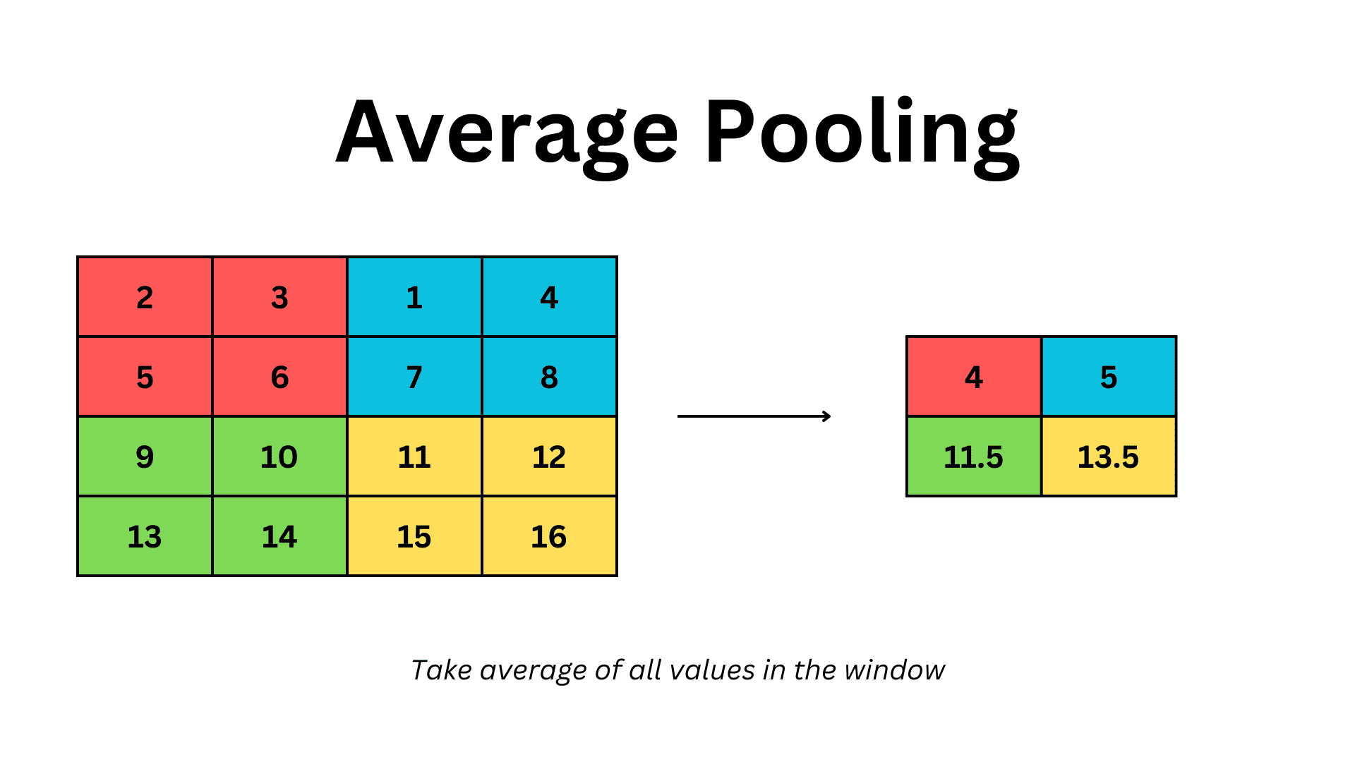
In average pooling, we similarly iterate over windows. However, we consider all values in the window, take the mean and then output that as our result.

Image by Author
Benefits of Average Pooling
- Preserving Spatial Information
In theory, we are retaining some information from all values in the window, to capture the central tendency of the activation values. In effect, we lose less information and can persist more spatial information from the convolutional activation values.
Averaging all values makes this method more robust to outliers relative to Max Pooling, as a single extreme value can not significantly alter the results of the pooling layer.
When taking the mean of values, we obtain less sharp transitions between our outputs. This provides a generalized representation of our data, allowing reduced contrast between subsequent layers.
Drawbacks
- Inability to Capture Salient Features
All values in a window are treated equally when the Average Pooling layer is applied. This fails to capture the dominant features from a convolutional layer, which can be problematic for some problem domains.
- Reduced Discrimination Between Features Maps
When all values are averaged, we can only capture the common features between regions. As such, we can lose the distinctions between certain features and patterns in an image, which is certainly a problem for tasks such as Object Detection.
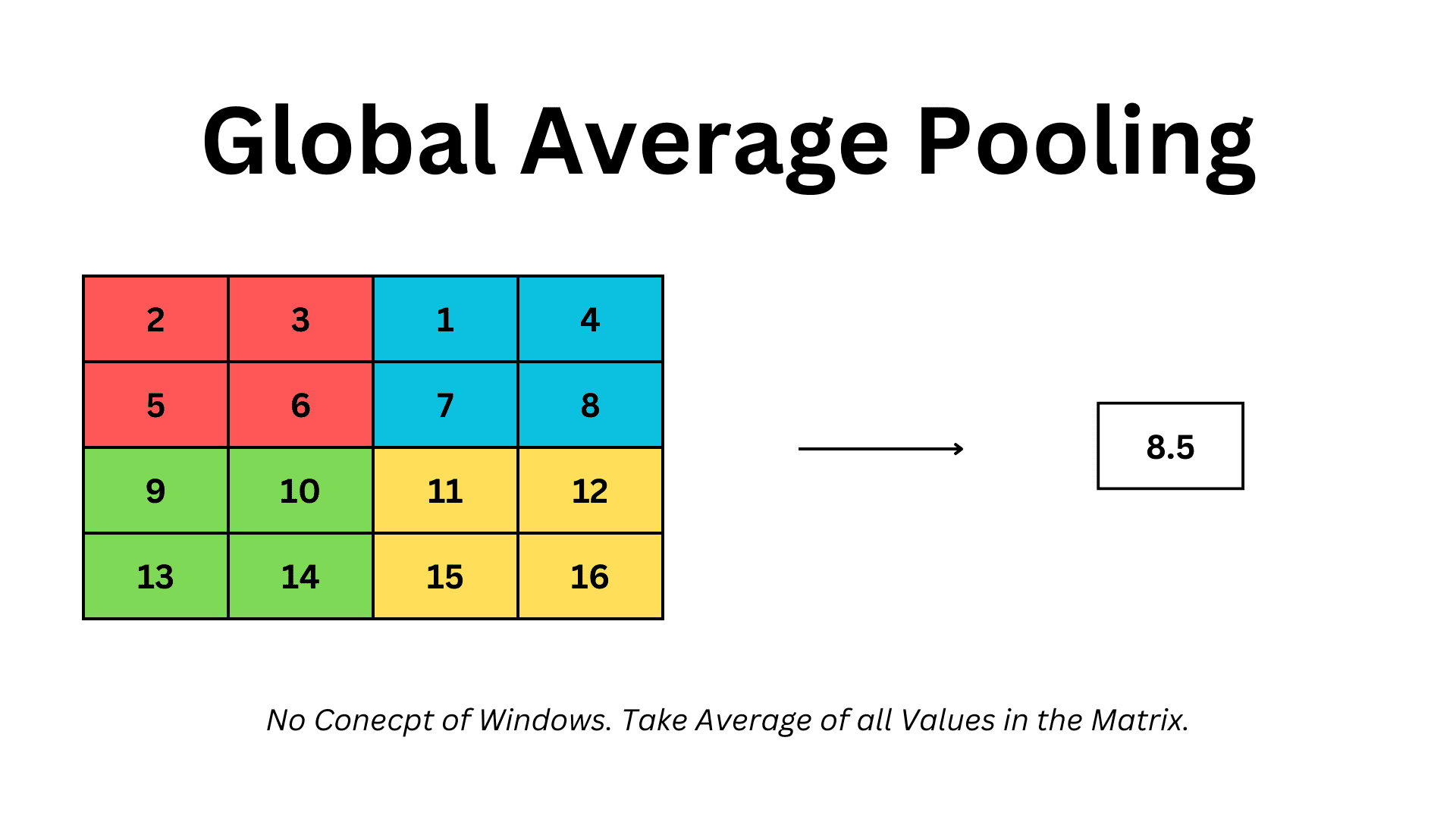
Global Pooling is different from normal pooling layers. It has no concept of windows, kernel size or stride. We consider the complete matrix as a whole and consider all values in the grid. In the context of the above example, we take the average of all values in the 4×4 matrix and get a singular value as our result.

Image by Author
When to Use
Global Average Pooling allows for straightforward and robust CNN architectures. With the use of Global Pooling, we can implement generalizable models, that are applicable to input images of any size. Global Pooling layers are directly used before dense layers.
The convolutional layers downsample each image, depending on kernel iterations and strides. However, the same convolutions applied to images of different sizes will result in an output of different shapes. All images are downsampled by the same ratio, so larger images will have larger output shapes. This can be a problem when passing it to Dense layers for classification, as size mismatch can cause runtime exceptions.
Without modifications in hyperparameters or model architecture, implementing a model applicable to all image shapes can be difficult. This problem is mitigated using Global Average Pooling.
When Global Pooling is applied before Dense layers, all input sizes will be reduced to a size of 1×1. So an input of either (5,5) or (50,50) will be downsampled to size 1×1. They can then be flattened and sent to the Dense layers without worrying about size mismatches.
We covered some fundamental pooling methods and the scenarios where each is applicable. It is critical to choose the one suitable for our specific tasks.
It is essential to clarify that there are no learnable parameters in pooling layers. They are simply sliding windows performing basic mathematical operations. Pooling layers are not trainable, yet they supercharge CNN architectures allowing faster computation and robustness in learning input features.
Muhammad Arham is a Deep Learning Engineer working in Computer Vision and Natural Language Processing. He has worked on the deployment and optimizations of several generative AI applications that reached the global top charts at Vyro.AI. He is interested in building and optimizing machine learning models for intelligent systems and believes in continual improvement.

