We have formally explained earlier the effect of class imbalance and its causes and we also explained several oversampling techniques that get around this issue such as random oversampling, ROSE, RWO, SMOTE, BorderlineSMOTE1, SMOTE-NC, and SMOTE-N. In this story, we will attempt to make a similar tour over undersampling techniques while assuming that it’s obvious how undersampling would help solve the imbalance issue given our earlier explanation.
Undersampling techniques generally fall into two main categories: controlled and uncontrolled. In controlled techniques, the algorithm receives a number that indicates how many samples there should be in the final dataset; meanwhile, in uncontrolled techniques undersampling is usually performed by simply removing points that meet some condition. It’s unknown a priori how many points will meet such condition and obviously it can’t be controlled. In this story, we will cover two controlled undersampling techniques (random and k-means undersampling) and two uncontrolled undersampling techniques (Tomek Links and Edited Nearest Neighbors).
Naive Random Undersampling
In this technique, if it’s given that N_k points should be removed from class k, then N_k points are randomly chosen from that class for deletion.
The following shows an example of undersampling the two majority classes in data with three classes 0, 1, and 2.
The following is an animation that shows the output at different degrees of undersampling
Notice how this is entirely a random process; no specific choice is made regarding which points to keep. The distribution of the data may be severely altered due to this.
K-Means Undersampling
We can preserve the distribution of the data by being more careful about which points to remove (or to keep). In K-means undersampling, if it is required to have N_k points for class k, then K-means is performed with K=N_k leading to N_k final centroids. K-means undersampling let’s those centers (or the nearest neighbor of each of them; this is a hyperparameter) be the final N_k points to return. Because the centers themselves preserve the distribution of the data, this results in a smaller set of points that preserve it as well.
The following shows an example of undersampling the two majority classes in data with three classes 0, 1, and 2.
Notice how it’s more careful in terms of preserving the structure of the data than random undersampling which would be even more evident with more undersampling. Let’s further illustrate this with an animation:
Note that the centers depend on the initialization which typically involves randomness.
Tomek Links Undersampling
This is an uncontrolled undersampling technique where a point can be removed if it is part of a Tomek link. Two points form a Tomek link if:
- They belong to different classes
- Each of the two points is the nearest neighbor of the other point
The rationale here is that such points don’t help make the decision boundary better (e.g., may make overfitting easier) and that they maybe noise. The following is an example for applying Tomek Links:
Notice how after undersampling it’s more easier to find a more linear decision boundary besides that this brings the data to better balance as well. In this, we skipped undersampling the minority class in green and stopped undersampling for a class once it had about as much points.
To see this in action more closely, where all classes are eventually undersampled, consider the following animation:
Edited Nearest Neighbors Undersampling
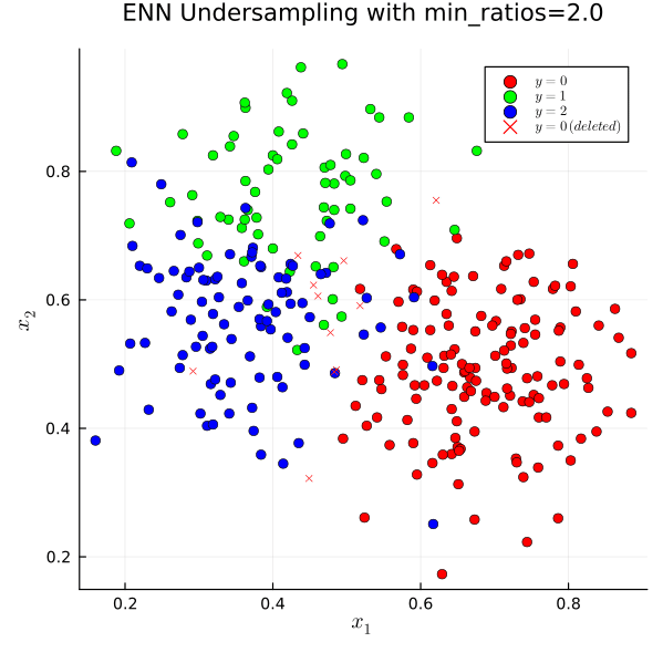
Although Tomek links are mostly points that don’t help form a better decision boundary or are noise, not all noisy points will form Tomek links. If a noisy point from class k_1 exists in a dense region in class k_2 then it can be normal for the nearest neighbor of the noisy point to have a nearest point that is not the noisy point which implies that it shall remain for not forming a Tomek link. Instead of this condition, edited nearest neighbors undersampling by default keeps a point iff the majority of its neighbors are from the same class. There is also the option to keep only if all of them are from the same class or for minimal undersampling to keep any point iff there exists a neighbor from the same class.
This animation portrays the algorithm in action:
Notice how it cleans out more points that would not be helpful to the decision boundary or are noise. Even more cleaning out can be done if the number of neighbors k or the keep condition is altered in the right way. This is another animation that illustrates the effect.
The difference between the “mode” and “only mode” conditions is that the former keeps a point iff its class is one of the most common among the neighbors; meanwhile, the latter keeps a point iff its class is the only most common class.
This wraps up our tour over some interesting undersampling algorithms. Hope this has helped you learn more about both controlled and uncontrolled undersampling. Till next time, au revoir.
References:
[1] Wei-Chao, L., Chih-Fong, T., Ya-Han, H., & Jing-Shang, J. (2017). Clustering-based undersampling in class-imbalanced data. Information Sciences, 409–410, 17–26.
[2] Ivan Tomek. Two modifications of cnn. IEEE Trans. Systems, Man and Cybernetics, 6:769–772, 1976.
[3] Dennis L Wilson. Asymptotic properties of nearest neighbor rules using edited data. IEEE Transactions on Systems, Man, and Cybernetics, pages 408–421, 1972.

