
Image by Author
Having a good title is crucial for an article’s success. People spend only one second (if we believe Ryan Holiday’s book “Trust Me, I’m Lying” deciding whether to click on the title to open the whole article. The media are obsessed with optimizing clickthrough rate (CTR), the number of clicks a title receives divided by the number of times the title is shown. Having a click-bait title increases CTR. The media will likely choose a title with a higher CTR between the two titles because this will generate more revenue.
I am not really into squeezing ad revenue. It is more about spreading my knowledge and expertise. And still, viewers have limited time and attention, while content on the Internet is virtually unlimited. So, I must compete with other content-makers to get viewers’ attention.
How do I choose a proper title for my next article? Of course, I need a set of options to choose from. Hopefully, I can generate them on my own or ask ChatGPT. But what do I do next? As a data scientist, I suggest running an A/B/N test to understand which option is the best in a data-driven manner. But there is a problem. First, I need to decide quickly because content expires quickly. Secondly, there may not be enough observations to spot a statistically significant difference in CTRs as these values are relatively low. So, there are other options than waiting a couple of weeks to decide.
Hopefully, there is a solution! I can use a “multi-armed bandit” machine learning algorithm that adapts to the data we observe about viewers’ behavior. The more people click on a particular option in the set, the more traffic we can allocate to this option. In this article, I will briefly explain what a “Bayesian multi-armed bandit” is and show how it works in practice using Python.
Multi-armed Bandits are machine learning algorithms. The Bayesian type utilizes Thompson sampling to choose an option based on our prior beliefs about probability distributions of CTRs that are updated based on the new data afterward. All these probability theory and mathematical statistics words may sound complex and daunting. Let me explain the whole concept using as few formulas as I can.
Suppose there are only two titles to choose from. We have no idea about their CTRs. But we want to have the highest-performing title. We have multiple options. The first one is to choose whichever title we believe in more. This is how it worked for years in the industry. The second one allocates 50% of the incoming traffic to the first title and 50% to the second. This became possible with the rise of digital media, where you can decide what text to show precisely when a viewer requests a list of articles to read. With this approach, you can be sure that 50% of traffic was allocated to the best-performing option. Is this a limit? Of course not!
Some people would read the article within a couple of minutes after publishing. Some people would do it in a couple of hours or days. This means we can observe how “early” readers responded to different titles and shift traffic allocation from 50/50 and allocate a little bit more to the better-performing option. After some time, we can again calculate CTRs and adjust the split. In the limit, we want to adjust the traffic allocation after each new viewer clicks on or skips the title. We need a framework to adapt traffic allocation scientifically and automatedly.
Here comes Bayes’ theorem, Beta distribution, and Thompson sampling.
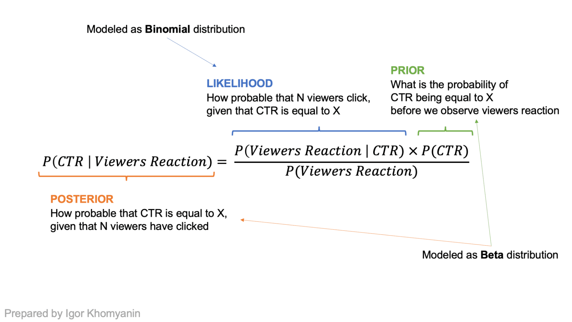
Let’s assume that the CTR of an article is a random variable “theta.” By design, it lies somewhere between 0 and 1. If we have no prior beliefs, it can be any number between 0 and 1 with equal probability. After we observe some data “x,” we can adjust our beliefs and have a new distribution for “theta” that will be skewed closer to 0 or 1 using Bayes’ theorem.
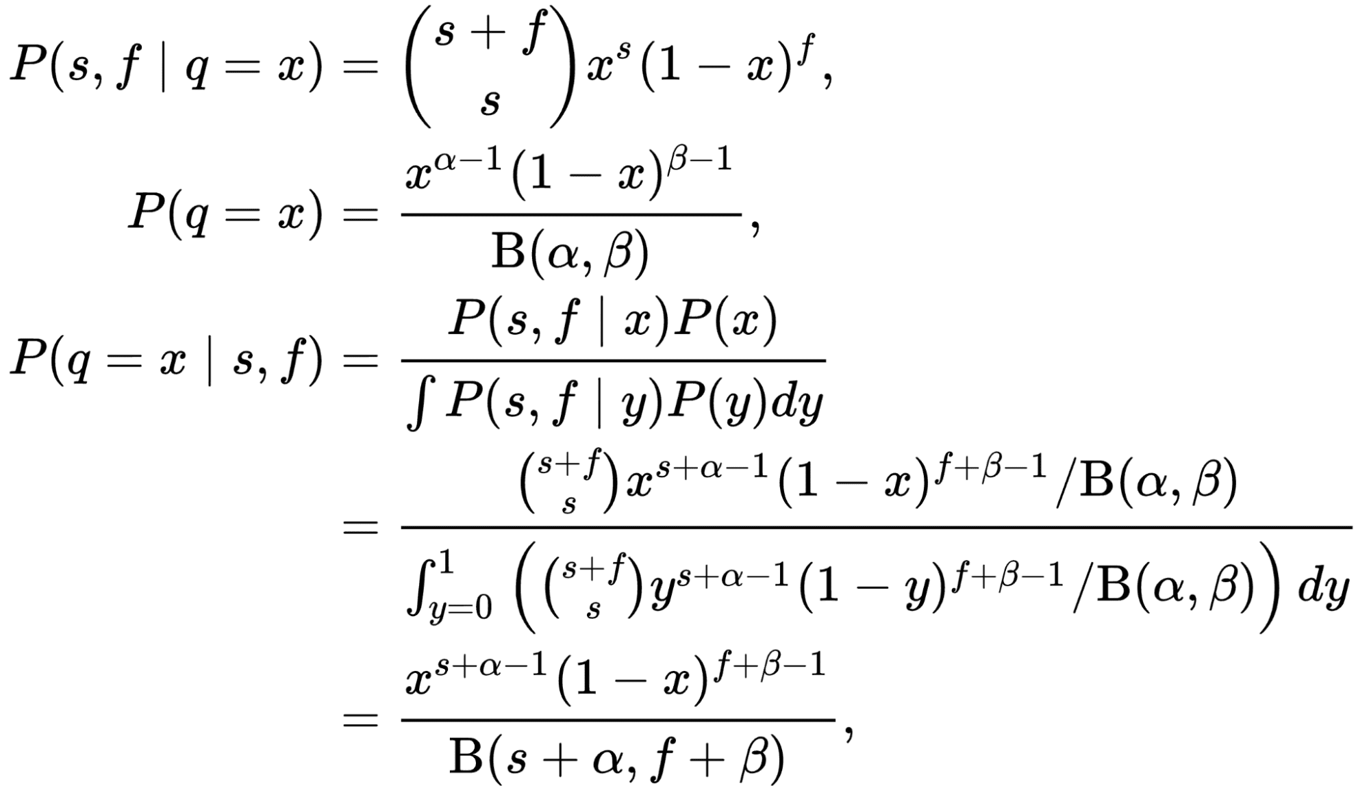
The number of people who click on the title can be modeled as a Binomial distribution where “n” is the number of visitors who see the title, and “p” is the CTR of the title. This is our likelihood! If we model the prior (our belief about the distribution of CTR) as a Beta distribution and take binomial likelihood, the posterior would also be a Beta distribution with different parameters! In such cases, Beta distribution is called a conjugate prior to the likelihood.
Proof of that fact is not that hard but requires some mathematical exercise that is not relevant in the context of this article. Please refer to the beautiful proof here:
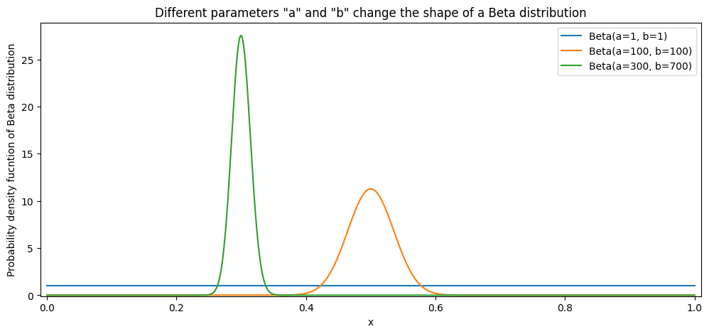
The beta distribution is bounded by 0 and 1, which makes it a perfect candidate to model a distribution of CTR. We can start from “a = 1” and “b = 1” as Beta distribution parameters that model CTR. In this case, we would have no beliefs about distribution, making any CTR equally probable. Then, we can start adding observed data. As you can see, each “success” or “click” increases “a” by 1. Each “failure” or “skip” increases “b” by 1. This skews the distribution of CTR but does not change the distribution family. It is still a beta distribution!
We assume that CTR can be modeled as a Beta distribution. Then, there are two title options and two distributions. How do we choose what to show to a viewer? Hence, the algorithm is called a “multi-armed bandit.” At the time when a viewer requests a title, you “pull both arms” and sample CTRs. After that, you compare values and show a title with the highest sampled CTR. Then, the viewer either clicks or skips. If the title was clicked, you would adjust this option’s Beta distribution parameter “a,” representing “successes.” Otherwise, you increase this option’s Beta distribution parameter “b,” meaning “failures.” This skews the distribution, and for the next viewer, there will be a different probability of choosing this option (or “arm”) compared to other options.
After several iterations, the algorithm will have an estimate of CTR distributions. Sampling from this distribution will mainly trigger the highest CTR arm but still allow new users to explore other options and readjust allocation.
Well, this all works in theory. Is it really better than the 50/50 split we have discussed before?
All the code to create a simulation and build graphs can be found in my GitHub Repo.
As mentioned earlier, we only have two titles to choose from. We have no prior beliefs about CTRs of this title. So, we start from a=1 and b=1 for both Beta distributions. I will simulate a simple incoming traffic assuming a queue of viewers. We know precisely whether the previous viewer “clicked” or “skipped” before showing a title to the new viewer. To simulate “click” and “skip” actions, I need to define some real CTRs. Let them be 5% and 7%. It is essential to mention that the algorithm knows nothing about these values. I need them to simulate a click; you would have actual clicks in the real world. I will flip a super-biased coin for each title that lands heads with a 5% or 7% probability. If it landed heads, then there is a click.
Then, the algorithm is straightforward:
- Based on the observed data, get a Beta distribution for each title
- Sample CTR from both distribution
- Understand which CTR is higher and flip a relevant coin
- Understand if there was a click or not
- Increase parameter “a” by 1 if there was a click; increase parameter “b” by 1 if there was a skip
- Repeat until there are users in the queue.
To understand the algorithm’s quality, we will also save a value representing a share of viewers exposed to the second option as it has a higher “real” CTR. Let’s use a 50/50 split strategy as a counterpart to have a baseline quality.
Code by Author
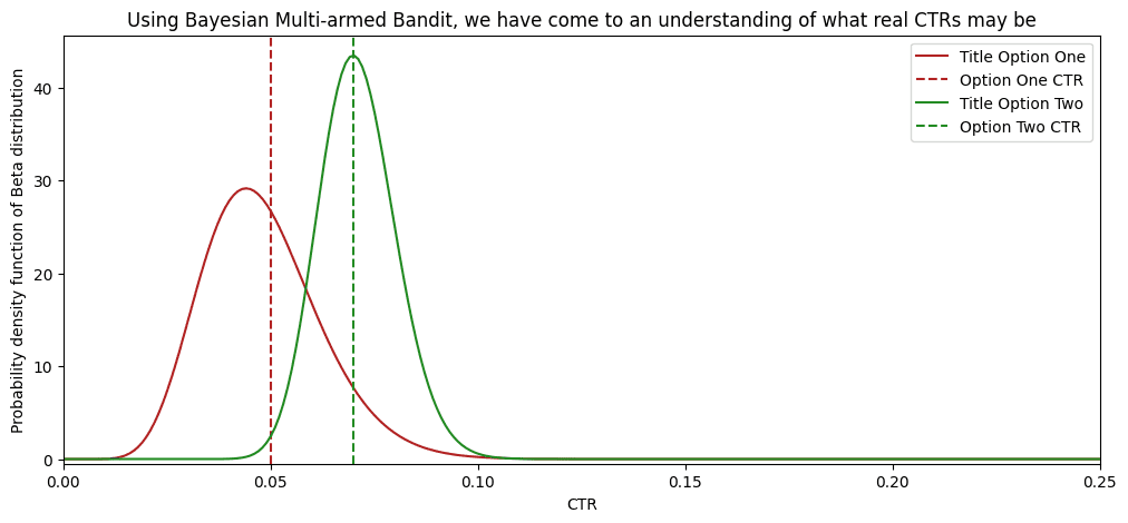
After 1000 users in the queue, our “multi-armed bandit” already has a good understanding of what are the CTRs.
And here is a graph that shows that such a strategy yields better results. After 100 viewers, the “multi-armed bandit” surpassed a 50% share of viewers offered the second option. Because more and more evidence supported the second title, the algorithm allocated more and more traffic to the second title. Almost 80% of all viewers have seen the best-performing option! While in the 50/50 split, only 50% of the people have seen the best-performing option.
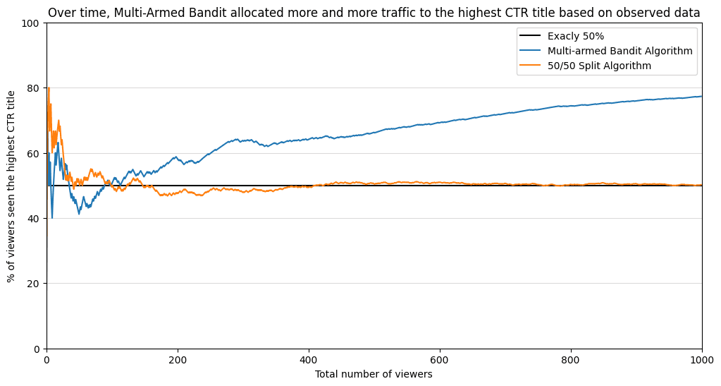
Bayesian Multi-armed Bandit exposed an additional 25% of viewers to a better-performing option! With more incoming data, the difference will only increase between these two strategies.
Of course, “Multi-armed bandits” are not perfect. Real-time sampling and serving of options is costly. It would be best to have a good infrastructure to implement the whole thing with the desired latency. Moreover, you may not want to freak out your viewers by changing titles. If you have enough traffic to run a quick A/B, do it! Then, manually change the title once. However, this algorithm can be used in many other applications beyond media.
I hope you now understand what a “multi-armed bandit” is and how it can be used to choose between two options adapted to the new data. I specifically did not focus on maths and formulas as the textbooks would better explain it. I intend to introduce a new technology and spark an interest in it!
If you have any questions, do not hesitate to reach out on LinkedIn.
The notebook with all the code can be found in my GitHub repo.
Igor Khomyanin is a Data Scientist at Salmon, with prior data roles at Yandex and McKinsey. I specialize in extracting value from data using Statistics and Data Visualization.

