Learn how a neural network with one hidden layer using ReLU activation can represent any continuous nonlinear functions.
Activation functions play an integral role in Neural Networks (NNs) since they introduce non-linearity and allow the network to learn more complex features and functions than just a linear regression. One of the most commonly used activation functions is Rectified Linear Unit (ReLU), which has been theoretically shown to enable NNs to approximate a wide range of continuous functions, making them powerful function approximators.
In this post, we study in particular the approximation of Continuous NonLinear (CNL) functions, the main purpose of using a NN over a simple linear regression model. More precisely, we investigate 2 sub-categories of CNL functions: Continuous PieceWise Linear (CPWL), and Continuous Curve (CC) functions. We will show how these two function types can be represented using a NN that consists of one hidden layer, given enough neurons with ReLU activation.
For illustrative purposes, we consider only single feature inputs yet the idea applies to multiple feature inputs as well.
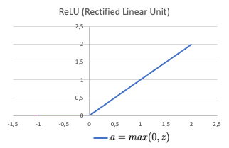
ReLU is a piecewise linear function that consists of two linear pieces: one that cuts off negative values where the output is zero, and one that provides a continuous linear mapping for non negative values.
CPWL functions are continuous functions with multiple linear portions. The slope is consistent on each portion, than changes abruptly at transition points by adding new linear functions.
In a NN with one hidden layer using ReLU activation and a linear output layer, the activations are aggregated to form the CPWL target function. Each unit of the hidden layer is responsible for a linear piece. At each unit, a new ReLU function that corresponds to the changing of slope is added to produce the new slope (cf. Fig.2). Since this activation function is always positive, the weights of the output layer corresponding to units that increase the slope will be positive, and conversely, the weights corresponding to units that decreases the slope will be negative (cf. Fig.3). The new function is added at the transition point but does not contribute to the resulting function prior to (and sometimes after) that point due to the disabling range of the ReLU activation function.
Example
To make it more concrete, we consider an example of a CPWL function that consists of 4 linear segments defined as below.
To represent this target function, we will use a NN with 1 hidden layer of 4 units and a linear layer that outputs the weighted sum of the previous layer’s activation outputs. Let’s determine the network’s parameters so that each unit in the hidden layer represents a segment of the target. For the sake of this example, the bias of the output layer (b2_0) is set to 0.
The next type of continuous nonlinear function that we will study is CC function. There is not a proper definition for this sub-category, but an informal way to define CC functions is continuous nonlinear functions that are not piecewise linear. Several examples of CC functions are: quadratic function, exponential function, sinus function, etc.
A CC function can be approximated by a series of infinitesimal linear pieces, which is called a piecewise linear approximation of the function. The greater the number of linear pieces and the smaller the size of each segment, the better the approximation is to the target function. Thus, the same network architecture as previously with a large enough number of hidden units can yield good approximation for a curve function.
However, in reality, the network is trained to fit a given dataset where the input-output mapping function is unknown. An architecture with too many neurons is prone to overfitting, high variance, and requires more time to train. Therefore, an appropriate number of hidden units should be large enough to properly fit the data and at the same time, small enough to avoid overfitting. Moreover, with a limited number of neurons, a good approximation with low loss has more transition points in restricted domain, rather than equidistant transition points in an uniform sampling way (as shown in Fig.10).
In this post, we have studied how ReLU activation function allows multiple units to contribute to the resulting function without interfering, thus enables continuous nonlinear function approximation. In addition, we have discussed about the choice of network architecture and number of hidden units in order to obtain a good approximation result.
I hope that this post is useful for your Machine Learning learning process!
Further questions to think about:
- How does the approximation ability change if the number of hidden layers with ReLU activation increases?
- How ReLU activations are used for a classification problem?
*Unless otherwise noted, all images are by the author

